Modelling steel strip heating within an annealing furnace

Abstract

Annealing furnaces are used to heat steel in order to change its chemical structure. In this paper we model an electric radiant furnace. One of the major defects in steel strips processed in such furnaces is a wave-like pattern near the edges of the strip, apparently due to extra heating near the edges. The aim of the paper is to model this effect and provide a way to calculate the elevated temperatures near the edges. We analyse two processes that are suspected to contribute to uneven heating. The modelling involves an asymptotic analysis of the effect of heat flux at the edges and a detailed analysis of the integral equations associated with radiant heat transfer in the furnace.

Introduction

The high temperatures within a steel annealing furnace preclude any reliable way to take measurements of the temperature; hence the need for mathematical models so that the temperature can be computed. We model an electric radiant annealing furnace with length of order 100 metres through which strips of steel sheet pass at speeds of up to 130 metres per minute in order to achieve the strip temperatures required for annealing. A schematic diagram of the furnace is shown in Fig. 4. The temperature along the furnace is controlled by varying the power supplied to the heating elements and the line speed through the furnace is reduced for strips of large thickness and width in order to achieve the required temperatures within the steel strips. At the beginning of the annealing–coating line there is an automatic welding process which welds the beginning of a new coil of steel sheet to the end of its predecessor, allowing the line to run continuously.

Occasionally the edges of the strip may take a wave-like shape after passing through the furnace and this seems to be a result of extra heating at the edges of the strip. This hypothesis is supported by a COMSOL^®; model of the system [1, 2] which shows a trend in increasing steel strip temperatures closer to the edges. The goal of this paper is to gain a better understanding of the nonuniform heating of the strip across its width.

The furnace has already been modelled in a recent Mathematics-in-Industry Study Group (MISG) meeting [5]. However the model developed in that meeting was based on an assumption of uniform heating across the width of the strip and is thus unsuitable for explaining such defects. There is a very limited amount of modelling of such furnaces in the literature. Apart from the papers already cited, perhaps the closest work is [10] which also takes into account the radiative heat transfer within a mullti-zone annealing furnace. However, although the model in [10] is more detailed than that given in [5], it also makes the approximation that the strip temperature does not vary across its width. Other related models concern an electric furnace model for crystal formation in the papers by Pérez-Grande et al. [7], Sauermann et al. [8], Teodorczyk and Januszkiewicz [9].

Because of the high temperatures within the furnace, radiant heat transfer is the primary mode of heat transfer. This is discussed briefly in the MISG paper [5], but for a complete discussion we cite some standard texts by Incropera and DeWitt [4], Modest [6], Siegel and Howell [3].

As a starting point to our modelling, we briefly summarise what was done in [5]. The temperature u of the steel strip is assumed to satisfy the heat equation

$$ \begin{aligned} \rho_{S} C_{S}\left(\frac{\partial u}{\partial t}+v \frac{\partial u}{\partial x}\right)=k_{S}\left(\frac{\partial^{2} u}{\partial x^{2}}\,+\,\frac{\partial^{2} u}{\partial y^{2}}\,+\,\frac{\partial^{2} u}{\partial z^{2}}\right), \,\,\,t\!>\!0, \,(x,y,z)\in \mathcal{S}, \end{aligned} $$

(1)

where

• the region of space occupied by the strip is

  $$ \mathcal{S}=\{(x,y,z): 0\le x\le L, -w/2\le y\le w, 0\le z\le h\}; $$

  (2)

• L is the length of the furnace;

• x measures distance from the point of entry of the strip into the furnace, z is a distance coordinate in the vertical direction and y is a distance coordinate across the strip;

• v is the velocity of the strip through the furnace;

• w and h are respectively the width and thickness of the strip.

• ρ _S , C _S and k _S are the strip’s density, specific heat capacity and heat conductivity respectively.

The functions w and h are typically piecewise constant functions of x and t and v can vary with time, but in this paper we limit our analysis to the desirable steady state operation of the furnace for which these variables are constant.

Equation 1 is supplemented by an initial condition

$$u(x,y,z,0)=u_{0}(x,y,z), \quad (x,y,z)\in \mathcal{S}, $$

and boundary conditions. It is assumed that the steel strip enters the furnace at x=0 at constant temperature T ₀, giving the Dirichlet boundary condition,

$$u(0,y,z,t)=T_{0}. $$

Mathematically, it is also appropriate to specify a boundary condition where the strip exits the furnace at x=L. One could propose a model leading to an appropriate boundary condition there. However we will see soon that heat conduction in the steel strip in the direction of the x-axis is very small, which means that the term involving $\frac {\partial ^{2} u}{\partial x^{2}}$ can be neglected everywhere except in a small boundary layer near x=L. Physically, heat is not conducted quickly enough for the temperature of the part of the strip that has already left the furnace to affect the temperature within the furnace. Thus, any boundary effect at x=L is not expected to be significant and thus we do not attempt to model it.

Boundary conditions on the remaining parts of the boundary of $\mathcal {S}$ arise from conservation of energy, which requires that we equate the normal component of the heat flux −k _S ∇u to the flux of radiant energy leaving the surface. Thus we write

$$ k_{S} \frac{\partial u}{\partial z}(x,y,h)=\phi_{a}(x,y), \quad k_{S} \frac{\partial u}{\partial z}(x,y,0)=-\phi_{b}(x,y), $$

(3)

for (x,y)∈(0,L)×(−w/2,w/2), and

$$ k_{S} \frac{\partial u}{\partial y}(x,w/2,z)\!=\phi_{c}(x,z), \quad \!\!k_{S} \frac{\partial u}{\partial y}(x,\!-w/2,z)=-\phi_{d}(x,z), $$

(4)

for (x,z)∈(0,L)×(0,h). The incoming surface heat fluxes ϕ _a , ϕ _b , ϕ _c and ϕ _d are determined by considering an energy balance of the radiation within the furnace.

We can determine the relative importance of the different terms in Eq. (1) by using dimensionless coordinates $\tilde {x}=x/L$, $\tilde {y}=y/w$, $\tilde {z}=x/h$, $\tilde {t}=tv/L$, where h and w are typical values of the thickness and width of the strip. In terms of the dimensionless variables, the equation takes the form

$$\frac{\partial u}{\partial \tilde{t}}+ \frac{\partial u}{\partial \tilde{x}}=\delta \left(\frac{w^{2}}{L^{2}}\frac{\partial^{2} u}{\partial \tilde{x}^{2}}+\frac{\partial^{2} u}{\partial \tilde{y}^{2}}+\frac{w^{2}}{h^{2}}\frac{\partial^{2} u}{\partial \tilde{z}^{2}}\right), $$

where

$$ \delta=\frac{k_{S} L}{v \rho_{S} C_{S} w^{2}}. $$

(5)

Taking the typical values L=150 m, v=2 m s ⁻¹, w=0.5 m, h=0.5 mm, k _S =50 W m ⁻¹ K ⁻¹, C _S =500 J Kg ⁻¹ K ⁻¹ and ρ _S =7854 Kg m ⁻³ gives δ=3.8×10⁻³ and the equation

$$ \frac{\partial u}{\partial \tilde{t}}+ \frac{\partial u}{\partial \tilde{x}}=4.2 \times 10^{-8}\frac{\partial^{2} u}{\partial \tilde{x}^{2}}+3.8 \times 10^{-3} \frac{\partial^{2} u}{\partial \tilde{y}^{2}}+3.8 \times 10^{3} \frac{\partial^{2} u}{\partial \tilde{z}^{2}}. $$

(6)

which was the justification in [5] for neglecting the heat conduction terms for the x and y directions in (1). Note however that boundary conditions must be satisfied, so one expects boundary layers near y=±w/2 where the boundary conditions are satisfied. We wish to investigate these particular boundary layers to see how much they contribute to edge heating. Thus we depart from the analysis in [5] by retaining the terms involving $\frac {\partial ^{2}u}{\partial y^{2}}$. However, as in [5], we neglect the term involving $\frac {\partial ^{2}u}{\partial x^{2}}$ and any associated boundary layer for reasons discussed earlier.

Thus (1) simplifies to

$$\begin{array}{*{20}l} \rho_{S} C_{S}\left(\! \frac{\partial u}{\partial t}\,+\,v \frac{\partial u}{\partial x}\!\right)&\!\,=\,k_{S}\!\left(\!\frac{\partial^{2} u}{\partial y^{2}}\,+\,\frac{\partial^{2} u}{\partial z^{2}}\!\right), \quad t>0, \,(x,y,z)\in \mathcal{S}. \end{array} $$

(7)

A further simplification results by considering the temperature of the strip averaged over the z-direction:

$$T(x,y,t)=\frac{1}{h}\int_{0}^{h} u(x,y,z,t)\,dz. $$

Equation (7) then leads to

$$ \rho_{S} C_{S}\left(\frac{\partial T}{\partial t}+v \frac{\partial T}{\partial x}\right) = k_{S}\frac{\partial^{2} u}{\partial y^{2}}+\frac{2\Phi_{S}}{h}, $$

(8)

where Φ _S is the average of the fluxes of heat entering the upper and lower surfaces of the strip:

$$\Phi_{S}=\frac{1}{2}\left[k\frac{\partial u}{\partial z}\right]_{z=0}^{z=h}=\frac{1}{2}(\phi_{a}+\phi_{b}). $$

Φ _S is calculated by considering the energy balance of the radiation within the furnace.

The relatively large coefficient of $\frac {\partial ^{2} u}{\partial \tilde {z}^{2}}$ in (6) indicates that we can use the approximation u(x,y,z,t)≈T(x,y,t) in our calculations. Thus we consider a model consisting of Eq. (8) with an initial condition

$$ T(x,y,0)=g(x,y), \quad 0<x<L, \quad -w/2<y<w/2, $$

(9)

and boundary conditions

$$\begin{array}{*{20}l} &T(0,y,t)=T_{0}, \quad t>0, \quad -w/2<y<w/2, \end{array} $$

(10)

$$\begin{array}{*{20}l} &\pm k_{S} \frac{\partial T}{\partial y}(x,\pm w/2)=\Phi_{E}^{\pm}, \quad 0<x<L, \end{array} $$

(11)

where $\Phi _{E}^{+}$ and $\Phi _{E}^{-}$ are the average radiant heat fluxes arriving at the edges of the strip.

$$\Phi_{E}^{+}(x)=\frac{1}{h}\int_{0}^{h} \phi_{d}(x,z)\,dz, \quad \Phi_{E}^{-}(x)=\frac{1}{h}\int_{0}^{h} \phi_{c}(x,z)\,dz. $$

The physical problem has reflectional symmetry through the x-z plane, so we assume that $\Phi _{E}^{+}=\Phi _{E}^{-}=\Phi _{E}.$

We wish to investigate two effects that could lead to edge heating of the strip. The first is the creation of a boundary layer near the edges y=±w/2 due to the boundary condition (11) there. We do this in Section 2. The second effect is a variation of Φ _S in the direction of the y-axis that might explain extra heating near the edges. This requires a detailed analysis of the radiation heat transfer problem to calculate Φ _S . We do this in Section 3. For the boundary layer analysis of Section 2 we use a simple approximation for Φ _S that is independent of y.

Analytical treatment of edge heating

The following approximate expression for Φ _S , the heat flux entering the upper and lower surfaces of the strip, was derived in [5].

$$\begin{array}{*{20}l} \Phi_{S}&= \frac{\epsilon_{S}\sigma\left(T_{W}^{4}-T_{1}^{4}\right)}{1+\frac{\epsilon_{S}(1-\epsilon_{W})}{\epsilon_{W}}\frac{w}{p}}, \end{array} $$

(12)

where ε _S ≈0.2 and ε _W ≈0.9 are the emissivities of the strip and furnace materials respectively, σ=5.670×10⁻⁸Wm⁻²K⁻⁴ is the Stefan–Boltzmann constant and p is the sum of height and width of a cross-section of the space inside the furnace. The temperature of the furnace walls and heating elements is assumed to be the same and is given by T _W . We note that this flux does not vary across the width of the strip. Smaller emissivities are associated with more reflective surfaces, which lead to a greater amount of reflection of radiant heat energy arriving at a surface.

Φ _E , the heat flux absorbed at the edges, is expected to be greater than Φ _S because the steel strips are formed by cold rolling of steel which results in a rougher, less reflective surface at the edges.

We limit our analysis to the steady state operation of the furnace. This simplifies the analysis because it allows us to approximate the heat flux Φ _S using the power supplied to the heating elements. For the non-steady state operation, one needs to take into account the heat dynamics that occur near the inner surface of the furnace walls, which are coupled to the dynamics of radiant heat transfer and heat transfer within the steel strip. For steady state operation, one can simply use the fact that the furnace walls are very good insulators and neglect the heat lost through them.

We thus seek steady state solutions of Eqs. (8), (10) and (11). In order to get a closed-form expression for the solution, we assume in Section 2.1 that ρ _S , C _S , k, Φ _S and Φ _E are all constant. We analyse the more general case for which these quantities are not constant in Section 2.2.

2.1 The case of constant ρ _S C _S , k, Φ _S and Φ _E

In terms of the dimensionless variables $\tilde {x}=x/L$, $\tilde {y}=y/w$, $\tilde {T}=T \frac {hv \rho _{S} C_{S}}{\Phi _{S} L}$, Eqs. (8), (10) and (11) become

$$\begin{array}{*{20}l} &\frac{\partial \tilde{T}}{\partial \tilde{x}}=\delta \frac{\partial^{2} \tilde{T}}{\partial \tilde{y}^{2}}+2, \end{array} $$

(13)

$$\begin{array}{*{20}l} &\tilde{T}(0,\tilde{y})=\tilde{T}_{0}, \end{array} $$

(14)

$$\begin{array}{*{20}l} &\frac{\partial \tilde{T}}{\partial \tilde{y}}(\tilde{x}, \pm 1/2)=\pm \frac{h}{w} \frac{\Phi_{E}}{ \Phi_{S}}\frac{1}{\delta}. \end{array} $$

(15)

Here, $\tilde {T}_{0}=T_{0} \frac {hv \rho _{S} C_{S}}{\Phi _{S} L}$ and δ is given by (5). In these equations, $0<\tilde {x}<1$ and $-1/2<\tilde {y}<1/2$.

We note that h/w and δ happen to be of the same order of magnitude for this industrial application, so the non-dimensional flux term in (15) is of order 1. This indicates that boundary edge heating is significant. However, δ is small, so we expect that the temperature of parts of the strip not close to the edges satisfies

$$\begin{array}{*{20}l} &\frac{\partial \tilde{T}_{1}}{\partial \tilde{x}}=2, \end{array} $$

(16)

$$\begin{array}{*{20}l} &\tilde{T}_{1}(0,\tilde{y})=\tilde{T}_{0}, \end{array} $$

(17)

which immediately gives

$$\tilde{T}_{1}(\tilde{x},\tilde{y})=\tilde{T}_{0}+2\tilde{x}. $$

We seek the steady state solution of the whole system (13)–(15), so we set $\tilde {T}=\tilde {T}_{0}+2\tilde {x}+\tilde {T}_{2}$ and see that $\tilde {T}_{2}$ must satisfy

$$\begin{array}{*{20}l} &\frac{\partial \tilde{T}_{2}}{\partial \tilde{x}}=\delta \frac{\partial^{2} \tilde{T}_{2}}{\partial \tilde{y}^{2}}, \end{array} $$

(18)

$$\begin{array}{*{20}l} &\tilde{T}_{2}(0,\tilde{y})=0, \end{array} $$

(19)

$$\begin{array}{*{20}l} &\frac{\partial \tilde{T}_{2}}{\partial \tilde{y}}(\tilde{x}, \pm 1/2)=\pm \frac{h}{w} \frac{\Phi_{E}}{ \Phi_{S}}\frac{1}{\delta}. \end{array} $$

(20)

We expect $\tilde {T}_{2}$ to remain close to zero, except in boundary layers near $\tilde {y}=\pm 1/2$, so we write $\tilde {y}=\delta ^{1/2}\zeta -1/2$. The scale factor δ ^1/2 for this inner variable ζ is chosen so that heating near the edge $\tilde {y}=-1/2$ is given by the equations

$$\begin{array}{*{20}l} &\frac{\partial \tilde{T}_{2}}{\partial \tilde{x}}=\frac{\partial^{2} \tilde{T}_{2}}{\partial \zeta^{2}}, \end{array} $$

(21)

$$\begin{array}{*{20}l} &\tilde{T}_{2}=0, \quad \text{for} \tilde{x}=0, \end{array} $$

(22)

$$\begin{array}{*{20}l} &\left.\frac{\partial \tilde{T}_{2}}{\partial \zeta}\right|_{\zeta=0}=-\frac{h}{w} \frac{\Phi_{E}}{ \Phi_{S}}\frac{1}{\delta^{1/2}}. \end{array} $$

(23)

Outside this boundary layer, the solution must match the outer solution and for this we use the simple matching condition $\tilde {T}_{2}\to 0$ as ζ→∞. The solution is easily obtained by taking the Laplace Transform with respect to the $\tilde {x}$ variable,

$$F(s,\zeta)=\int_{0}^{\infty} \tilde{T}_{2}(\tilde{x},\tilde{y})e^{-s\tilde{x}}\,d\tilde{x}, \quad \text{with} \tilde{y}=\delta^{1/2}\zeta-1/2. $$

Equation 21 then gives sF=F _{ζ ζ} , from which we find that

$$F(s,\zeta)=\frac{h}{w} \frac{\Phi_{E}}{ \Phi_{S}}\frac{1}{\sqrt{s^{3} \delta}}e^{-\sqrt{s} \zeta}. $$

This gives

$$ \tilde{T_{2}}= \frac{1}{\sqrt{\delta}}\frac{h}{w} \frac{\Phi_{E}}{ \Phi_{S}}\psi(\zeta,\tilde{x})=\frac{1}{\sqrt{\delta}}\frac{h}{w} \frac{\Phi_{E}}{ \Phi_{S}}\psi\left(\frac{\tilde{y}+1/2}{\sqrt{\delta}},\tilde{x}\right), $$

(24)

where

$$ \psi(\zeta,\tilde{x})= \zeta\left(\text{erf}\left(\frac{\zeta}{2\sqrt{\tilde{x}}}\right)-1\right) + 2\sqrt{\frac{\tilde{x}}{\pi}}\exp\left(\frac{-\zeta^{2}}{4\tilde{x}}\right), $$

(25)

and erf represents the error function,

$$\text{erf}(z)=\frac{2}{\sqrt{\pi}}\int_{0}^{z} e^{-s^{2}}\,ds. $$

A similar expression approximates the boundary layer near $\tilde {y}=1/2$. One can combine the inner and outer solutions to obtain a composite approximation for the steady state solution of (13)–(15), valid for −1/2≤y≤1/2:

$$\tilde{T}\,=\,\tilde{T}_{0}+2\tilde{x}+\frac{1}{\sqrt{\delta}}\frac{h}{w} \frac{\Phi_{E}}{ \Phi_{S}}\left(\!\psi\!\left(\frac{\tilde{y}+1/2}{\sqrt{\delta}},\tilde{x}\right) \,+\,\psi\!\left(\!\frac{1/2-\tilde{y}}{\sqrt{\delta}},\tilde{x}\right)\right) $$

In terms of the original variables, one finds that the boundary layer penetrates to a distance

$$2\sqrt{\frac{k_{S} x}{v \rho_{S} C_{S}}} $$

and the increased temperature at the edge is

$$\Phi_{E}\sqrt{\frac{x}{\pi k_{S} v \rho_{S} C_{S}}}. $$

We use these equations to plot an example of increased strip temperature near an edge in Fig. 1. The calculations for the figure use Φ _E =Φ _S but in fact we expect Φ _E >Φ _S because the upper and lower surfaces are very smooth and are thus expected to have a lower emissivity than the edge surfaces. Thus we expect the edge temperatures to be greater than those shown in the graphs. Also used in the calculations are the values k _S =50 Wm ⁻¹ K ⁻¹, C _S =500 JK ⁻¹ Kg ⁻¹, T ₀=573 K, ρ _S =7854 Kgm ⁻³, h=0.5 mm, w=0.5 m, v=2 ms ⁻¹, L=100 m, Φ _E =Φ _S =1500 Wm ⁻².

Fig. 1

The effect of radiation arriving at an edge. The actual effect is expected to be greater than this because of the higher emissivity of the edges

2.2 The case of variable ρ _S , C _S , k, Φ _S and Φ _E

In this section, we wish to follow the analysis of Section 2.1, but now in the more realistic setting of variable ρ _S , C _S , k, Φ _S and Φ _E . In practice, the large temperature variation within annealing furnaces requires that we take into account the temperature variation, especially of C _S and k _S , and to a lesser extent, ρ _S . The variation of C _S and k _S with temperature, shown in Figs. 2 and 3, is taken from data in [4]. Figure 3 shows that heat conductivity is approximated well using linear regression:

$$ k_{S}=73.9823-0.0437 T, $$

(26)

Fig. 2

Variation of C _p (J/Kg.K) for steel with absolute temperature T in Kelvin

Fig. 3

Variation of the heat conductivity k (W/m.K) for steel with absolute temperature T in Kelvin

and Fig. 2 shows the C _p data approximated by an interpolating quartic:

$$ \begin{aligned} C_{S} &=345 - 0.504333T + 0.004895T^{2} \\ &- 9.06667{\times10}^{-6}T^{3} + 5.5{\times10}^{-9}T^{4}. \end{aligned} $$

(27)

To allow for such variations, we assume that ρ _S , C _S and k _S are known functions of the strip’s temperature. Further, because our system is at equilibrium, Φ _S and Φ _E are assumed to be known functions of x which can be calculated by measuring the power supplied to the heating elements in the vicinity of a distance x along the furnace.

The form of Eq. (1) is only valid for constant diffusivity k _S . With variable k _S , we must instead write

$$ \rho_{S} C_{S}\left(\frac{\partial u}{\partial t}+v \frac{\partial u}{\partial x}\right)=\nabla \cdot (k_{S} \nabla u). \quad \text{in} \mathcal{S}\times(0,\infty). $$

(28)

Consequently, instead of (8), we have

$$ \rho_{S} C_{S}\left(\frac{\partial T}{\partial t}+v \frac{\partial T}{\partial x}\right) = \frac{\partial}{\partial y}\left(k_{S}\frac{\partial T}{\partial y}\right)+\frac{2\Phi_{S}}{h}. $$

(29)

Hence the steady state temperature must satisfy

$$\begin{array}{*{20}l} &\rho_{S} C_{S} v \frac{\partial T}{\partial x} = k_{S}(T)\frac{\partial^{2} T}{\partial y^{2}}+k_{S}'(T)\left(\frac{\partial T}{\partial y}\right)^{2}+\frac{2\Phi_{S}}{h}, \end{array} $$

(30)

$$\begin{array}{*{20}l} &T(0,y)=T_{0}, \quad -w/2<y<w/2, \end{array} $$

(31)

$$\begin{array}{*{20}l} &\pm k_{S} \frac{\partial T}{\partial y}(x,\pm w/2)=\Phi_{E}, \quad 0<x<L. \end{array} $$

(32)

As before, the small diffusivity indicates that for y not close to ±w/2, T(x,y)≈T ₁(x), where T ₁ satisfies the ordinary differential equation

$$ \rho_{S}(T_{1})C_{S}(T_{1})v T_{1}'(x)=\frac{2\Phi_{S}(x)}{h},\quad T_{1}(0)=T_{0}. $$

(33)

As before, it is useful to consider a new dimensionless variable $\tilde {x}$, this time chosen to make the coefficients of Eq. (32) more similar to those of the constant coefficient case. We do this by choosing $\tilde {x}$ to be the solution to

$$L\frac{d\tilde{x}}{dx}= \frac{k_{S}(T_{1})\rho_{S}(T_{0})C_{S}(T_{0})}{k_{S}(T_{0})\rho_{S}(T_{1})C_{S}(T_{1})}, \quad \tilde{x}(0)=0, $$

where T ₁=T ₁(x). We also let $\tilde {y}=y/w$.

In terms of these variables, Eq. (30) takes the form

$$ \begin{aligned} \frac{\!k_{S}(\!T_{1}\!)\!\rho_{S}\!(\!T)C_{S}(T)}{k_{S}(\!T)\!\rho_{S}(\!T_{1})C_{S}(\!T_{1})}\frac{\partial T}{\!\partial \tilde{x}}\,=\,\delta\frac{\partial^{2} T}{\partial \tilde{y}^{2}}\,+\,\delta \frac{k_{S}'(T)}{k_{S}(T)}\!\left(\!\frac{\partial T}{\partial \tilde{y}}\!\right)^{2}\!\,+\,\frac{2\Phi_{S} k_{S}(\!T_{0}\!)L}{h v \rho_{S}(\!T_{0})C_{S}(\!T_{0})k_{S}(\!T)}, \end{aligned} $$

(34)

where δ is again given by Eq. (5), but with k _S , ρ _S and C _S evaluated at temperature T ₀. Finally, we choose a dimensionless temperature

$$\tilde{T}=T\frac{h v \rho_{S}(T_{0})C_{S}(T_{0})}{\overline{\Phi}_{S} L}, $$

where $\overline {\Phi }_{S}$ is the average of Φ _S ,

$$\overline{\Phi}_{S}=\frac{1}{L}\int_{0}^{L} \Phi_{S}(x)\,dx. $$

Equation 34 becomes

$$ \begin{aligned} \frac{k_{S}(T_{1})\rho_{S}(T)C_{S}(T)}{k_{S}(T_{0})\rho_{S}(T_{1})C_{S}(T_{1})}\frac{\partial \tilde{T}}{\partial \tilde{x}}&= \\ \frac{k_{S}(T)}{k_{S}(T_{0})}\delta\frac{\partial^{2} \tilde{T}}{\partial \tilde{y}^{2}}&+\delta \frac{\overline{\Phi}_{S} L}{h v \rho_{S}(T_{0})C_{S}(T_{0}\!)} \frac{k_{S}'(T)}{k_{S}(T_{0})}\!\!\left(\!\frac{\partial \tilde{T}}{\partial \tilde{y}}\!\right)^{2}\!\,+\,\frac{2\Phi_{S}}{\overline{\Phi}_{S} }\!. \end{aligned} $$

(35)

The dimensionless solution of Eq. (35) corresponding to the solution T ₁ of Eq. (33) is given by

$$\tilde{T}_{1}(\tilde{x})=\frac{T_{1}(x)}{\overline{T}}, \quad \text{where} \quad \overline{T}=\frac{\overline{\Phi}_{S} L}{h v \rho_{S}(T_{0})C_{S}(T_{0})}, $$

and this corresponds to a solution outside boundary layers.

As in Section 2.1, we set $\tilde {y}=\delta ^{1/2}\zeta -1/2$; ζ is our boundary layer variable near the edge $\tilde {y}=-1/2$. We also write $\tilde {T}=\tilde {T}_{1}(\tilde {x})+\tilde {T}_{2}(\tilde {x},\zeta)$. Rewriting the boundary condition (32) at this edge in terms of the new variables gives

$$ \left.\frac{\partial \tilde{T}_{2}}{\partial \zeta}\right|_{\zeta=0}=-\frac{h}{w} \frac{\Phi_{E} k_{S}(T_{0})}{ \overline{\Phi}_{S} k_{S}(T)}\frac{1}{\delta^{1/2}}. $$

(36)

It is very desirable for the industrial application that edge heating is very small. This is consistent with our observation that the physical parameters happen to be such that h/w=O(δ), and thus the right-hand-side of (36) is O(δ ^1/2). In any case, we assume that

$$\frac{h}{w}\delta^{-1/2}=\epsilon $$

is small and we write $\tilde {T}_{2}(\tilde {x},\zeta)=\epsilon \theta (\tilde {x},\zeta)+O(\epsilon ^{2})$. This allows us to use a first order Taylor approximation to ρ _S (T), expanded about the point T=T ₁,

$$\rho_{S}(T)=\rho_{S}(T_{1})+\epsilon \rho_{S}'(T_{1})\overline{T}\theta(\tilde{x},\zeta)+O(\epsilon^{2}). $$

We use similar approximations for C _S (T) and k _S (T).

Recalling that $\partial /\partial \tilde {y}=\delta ^{-1/2} \partial /\partial \zeta$, we expand Eq. (35) up to O(ε) to find that θ must satisfy

$$ \left(\frac{\rho_{S}'(T_{1})}{\rho_{S}(T_{1})}+\frac{C_{S}'(T_{1})}{C_{S}(T_{1})}\right)\frac{\partial T_{1}}{\partial \tilde{x}}\theta+\frac{\partial \theta}{\partial \tilde{x}}=\frac{\partial^{2} \theta}{\partial \zeta^{2}}. $$

(37)

Equation 37 may be simplified by setting

$$ \chi=\frac{\rho_{S}(T_{1})C_{S}(T_{1})}{\rho_{S}(T_{0})C_{S}(T_{0})}\theta, $$

(38)

and we find that χ satisfies

$$ \frac{\partial \chi}{\partial \tilde{x}}=\frac{\partial^{2} \chi}{\partial \zeta^{2}}. $$

(39)

The flux boundary condition (36) translates to

$$ \left.\frac{\partial \chi}{\partial \zeta}\right|_{\zeta=0}=-\frac{\Phi_{E}}{\overline{\Phi}_{S}}\frac{k_{S}(T_{0})\rho_{S}(T_{1})C_{S}(T_{1})}{k_{S}(T_{1})\rho_{S}(T_{0})C_{S}(T_{0})}=f(\tilde{x}). $$

(40)

χ must also satisfy an “initial” condition, χ(0,ζ)=0, and a matching condition, $\chi (\tilde {x},\zeta)\to 0$ as ζ→∞.

The solution of this system, readily found by use of the Laplace transform, is

$$ \chi(\tilde{x},\zeta)=\int_{0}^{\tilde{x}} g(\zeta,\sigma)f(\tilde{x}-\sigma)\,d\sigma, $$

(41)

where $g(\zeta,\tilde {x})=\frac {\partial \psi }{\partial \tilde {x}}=e^{-\zeta ^{2}/4\tilde {x}}/\sqrt {\pi \tilde {x}}$ and ψ is given by Eq. (25).

In summary, we have found that there is a boundary layer near the edges of the strip. Outside the boundary layer, the temperature T ₁ of the strip, at a distance x along the furnace, may be found by solving the ordinary differential Eq. (33). With T ₁(x), we may then calculate $f(\tilde {x})$ from (40) and then χ from (41). This gives us θ from (38). The actual perturbation to the temperature near the edge y=−w/2 is given by

$$T_{2}=\overline{T}\tilde{T_{2}}=\overline{T}\epsilon \theta(\tilde{x},\zeta). $$

Furnace radiative heat transfer analysis

3.1 Assumptions

The radiative heat exchange between the furnace inner surface and the strip is considered in this section. The schematic geometry of the problem is presented in Fig. 4 which shows the cross section and the side view of the furnace and the strip. The furnace is modelled as a hollow rectangular box with length much larger than the dimensions of the cross section. The heating elements are assembled on the top and bottom inner surfaces of the furnace. We make the following assumptions about the radiative heat transfer within the furnace.

Fig. 4

Sketch of the furnace; a cross-section, b side view

• 1. The heating elements are distributed uniformly over the top and bottom inner surfaces and the the density of the input electric power is specified as a constant.

• 2. All surfaces are considered opaque gray. All surfaces emit and reflect radiation diffusely; the typical emissivity of the furnace wall surface and the heating element is ε _W =ε _E =0.9 and of the strip is ε _S =0.2. For an opaque gray surface, the reflectivity ρ and emissivity ε are related by ρ=1−ε.

• 3. Temperature changes within the furnace are gradual and radiative and thus convective heat transfer along the length of the furnace can be ignored. The strip temperature at the entry of the furnace is at room temperature and it can reach up to 700 °C at the last heating stage, which is still significantly lower than the temperature of wall surface and the heating elements. Considering that the radiative power is proportional to the fourth power of the temperature, the dominant radiation is from the wall surfaces and the heating elements.

These assumptions simplify the analysis and are reasonable for a furnace with brick covered wall and a steel strip with rough surface finishing. For a steel strip with smooth surface finishing, a partly specular reflection model shall be considered.

We use these assumptions to develop a two dimensional model of the temperature distribution within the furnace. The model is two dimensional only in the sense that it relies on the approximation that there is only a gradual variation of temperature in the direction of the moving strip.

We are interested in temperature variations across the strip and for this we must solve a system of integral equations for the radiative and reflective heat exchange between surfaces within the furnace.

3.2 Mathematical model

For a diffuse surface, it is well known that the net radiation method can be used to analyse the heat transfer. This method is discussed in many texts on thermal radiation such as the works of Modest [6] and of Siegel and Howell [3]. The method, which involves an energy conservation argument for the absorption, emission and reflection of radiation inside an enclosure, results in an integral equation.

Let q(x) be the outgoing heat flux at the location x, which counts both radiant and reflected heat fluxes. The governing integral equation in terms of q(x) takes the form

$$\begin{array}{@{}rcl@{}} q(\mathbf{x})=\epsilon (\mathbf{x})\sigma T^{4}(\mathbf{x})+\rho(\mathbf{x})\int_{A} q(\mathbf{x'})dF_{d \mathbf{x} - d \mathbf{x'}}, \end{array} $$

(42)

for surfaces where the temperature T(x) is given, or

$$\begin{array}{@{}rcl@{}} q(\mathbf{x})=p(\mathbf{x})+ \int_{A} q(\mathbf{x'})dF_{d \mathbf{x} - d \mathbf{x'}}, \end{array} $$

(43)

for the surfaces where the input power flux p(x) is specified. In the integral equation ρ(x) is the reflectance of the surface at x and $\phantom {\dot {i}\!}dF_{d \mathbf {x} - d \mathbf {x}^{\prime } }$ is the exchange view factor between two surface elements d x and dx ^′, which is defined as,

$$ {\begin{aligned} {\kern-16.5pt}{dF}_{d\mathbf{x}-d\mathbf{x}^{\prime}} \!\equiv\! \frac{\text{diffuse energy leaving} d \text{x directly toward and intercepted by d}~\mathbf{x}^{\prime}} {\text{total diffuse energy leaving d}~\mathbf{x}}\!. \end{aligned}} $$

(44)

Note that d x denotes the differential strip element which, due to the longitudinal symmetry, is infinite in the x ₃ direction.

The diffuse view factor between two infinitesimal strip elements d x, dx ^′ located at x and x ^′ respectively, as shown in Fig. 5, is given by

$$ \begin{aligned} {d \mathbf{x} - d \mathbf{x'} }\,=\, \frac{\cos \beta \sin \beta d \mathbf{x'} }{2r}\,=\,\frac{|(x_{1} -x_{1}')(x_{2} -x_{2}') | d \mathbf{x'} }{2 \left((x_{1} -x_{1}')^{2} + (x_{2} -x_{2}')^{2}\right)^{3/2} } \end{aligned} $$

(45)

Fig. 5

Diagram for calculation of view factors

for perpendicular elements and

$$ \begin{aligned} dF_{d \mathbf{x} - d \mathbf{x'} }= \frac{\sin^{2} \beta d \mathbf{x'} }{2r} = \frac{d^{2} d \mathbf{x'} }{2((x_{1} -x_{1}')^{2} + (x_{2} -x_{2}')^{2})^{3/2} } \end{aligned} $$

(46)

for parallel elements, where β are the angles shown in Fig. 5, d is the perpendicular distance between the two parallel elements, see [3].

We define the kernel k(x,x ^′) to be zero if the points x and x ^′ are shielded from each other by another surface, otherwise it is given by

$$ \begin{aligned} k(\mathbf{x},\mathbf{\!x'})\,=\,\!\left\{\!\!\! \begin{array}{ll} \frac{|(x_{1} \,-\,x_{1}')(x_{2} \,-\,x_{2}') | }{2((x_{1} \,-\,x_{1}')^{2} + (x_{2} -x_{2}')^{2})^{3/2} }, & \text{\!\!if x and x' are on perpendicular elements,} \\ \frac{d^{2}}{2((x_{1} -x_{1}')^{2} + (x_{2} -x_{2}')^{2})^{3/2} }, & \text{\!\!if x and x' are on parallel elements.} \end{array} \right. \end{aligned} $$

(47)

The integral equation can be written via kernel k(x,x ^′)

$$\begin{array}{@{}rcl@{}} q(\mathbf{x})=\epsilon(\mathbf{x}) \sigma T^{4}(\mathbf{x})+\rho(\mathbf{x})\int_{A}q(\mathbf{x'}) k(\mathbf{x},\mathbf{x'}) d\mathbf{x'} \end{array} $$

(48)

for a surface where the temperature is given, or

$$\begin{array}{@{}rcl@{}} q(\mathbf{x})=p(\mathbf{x})+\int_{A} q(\mathbf{x'})k(\mathbf{x},\mathbf{x'}) d\mathbf{x'} \end{array} $$

(49)

for a surface where the input power flux is given. The integral equation uniquely determines the outgoing heat flux q(x).

3.3 Numerical procedure

In general such integral equations do not have a closed form solution so a numerical method is needed to find an approximate solution. The integral equation is linear and the discretised equation is a linear system and can be solved by a standard LU decomposition. To numerically solve (48) and (49), all of the surfaces, which because of the assumption of longitudinal symmetry of the problem, are one dimensional domains, are divided into sufficiently small intervals of equal length and the q(x) is assigned on the nodes q(x _i ). A standard trapezoid method is applied to integrate (48) and (49) numerically, resulting in a linear system with q(x _i ) as unknowns.

In the actual numerical procedure, however, care must be taken in the treatment of discontinuities and singularities arising from the singularity of the kernel k(x,x ^′). Let us consider why these arise.

• 1. The k(x,x ^′) function has a discontinuity at the corner points of the wall arising from the two different formulas for the parallel and perpendicular elements. Thus, the numerical integration is performed on the individual planar surfaces. This gives a total of six planar surfaces including four wall surfaces and two strip surfaces.

• 2. For a node x located on a furnace wall, the kernel k(x,x ^′) is only a piecewise smooth function of x ^′ due to the presence of the steel strip and its shadow effect.

  This can be observed from Fig. 6, showing a node x exposed only to partial heat flux emitted from another wall surface. The kernel k(x,x ^′) has jumps at x1′ and x2′, each of which lies between two neighboring nodes. The exact positions of x1′ and x2′ can be found from the geometric relation. The numerical integration is performed only on the viewable portion of the relevant subintervals bounded by x1′ (or x2′) and one of the two neighboring nodes.

• 3. Due to the singularity of the kernel k(x,x ^′), when two nodes on the neighboring wall are sufficiently close, the variation of k(x,x ^′) on a single element is significant for whatever small step size has been chosen. To overcome this singularity, the following approximation is applied to these nodes.

  Fig. 6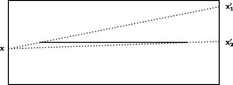

  

  Shadow effect of the strip

  Assuming a linear distribution of the q(x) on the element (xi′,xi+1′), we may estimate the integral in (48) and (49) as

  $$ \begin{aligned} \int_{\mathbf{x}_{i}'}^{\mathbf{x}_{i+1}'} q(\mathbf{x'}) k(\mathbf{x},\mathbf{x'}) d\mathbf{x'} \approx \frac{1}{h } \int_{\mathbf{x}_{i}'}^{\mathbf{x}_{i+1}'} ((q(\mathbf{x}_{i+1}')\\-q(\mathbf{x}_{i}'))| \mathbf{x'} - \mathbf{x}_{i}'|+ q(\mathbf{x}_{i}')h) k(\mathbf{x},\mathbf{x'}) d\mathbf{x'} \end{aligned} $$

  (50)

  where h=|xi′−xi+1′| is the step size. This can be written in terms of q(x _i+1) and q(x _i )

  $$\begin{array}{@{}rcl@{}} \int_{\mathbf{x}_{i}'}^{\mathbf{x}_{i+1}'} q(\mathbf{x'}) k(\mathbf{x},\mathbf{x'}) d\mathbf{x'} \approx C_{i}^{(1)} q(\mathbf{x}_{i}') + C_{i}^{(2)} q(\mathbf{x}_{i+1}') \end{array} $$

  where the coefficients $C_{i}^{(1)}$ and $C_{i}^{(2)}$ are determined by

  $$\begin{array}{@{}rcl@{}} C_{i}^{(1)}= \frac{1}{h}\int_{\mathbf{x}_{i}'}^{\mathbf{x}_{i+1}'}(h- | \mathbf{x}'-x_{i}'|) k(\mathbf{x},\mathbf{x'}) d\mathbf{x'}. \end{array} $$

  (51)

  and

  $$\begin{array}{@{}rcl@{}} C_{i}^{(2)}= \frac{1}{ h}\int_{\mathbf{x_{i}'}}^{\mathbf{x_{i+1}'}} | \mathbf{x'-x_{i}'}| k(\mathbf{x},\mathbf{x'}) d\mathbf{x'}, \end{array} $$

  (52)

  respectively. Adding the l corner elements leads to

  $$ \begin{aligned} {\sum_{i=1}^{l}} \frac{1}{h } \int_{\mathbf{x_{i}'}}^{\mathbf{x_{i+1}'}} ((q(\mathbf{x_{i+1}'})-q(\mathbf{x_{i}'}))| \mathbf{x'} - \mathbf{x_{i}'}|+ q(\mathbf{x_{i}'})h) k(\mathbf{x},\mathbf{x'}) d\mathbf{x'} \\ = C_{1}^{(1)}q(\mathbf{x_{1}'}) +C_{l}^{(2)}q(\mathbf{x_{l+1}'}) + \sum_{i=2}^{l-1} (C_{i}^{(1)}+C_{i-1}^{(2)})q(\mathbf{x_{i}'}) \end{aligned} $$

  (53)

  l will be chosen to cover all elements affected by the kernel singularity.

• 4. There are two nodes belonging to two neighbouring walls intersecting at a corner point denoted by $\mathbf {x_{S_{1}}}$ and $\mathbf {x_{S_{2}}}$ where S ₁ and S ₂ indicate the surfaces the nodes belong to. The integration with respect to x ^′ over the surface S ₂ for $\mathbf {x} = \mathbf {x_{S_{1}}}$ should be estimated by calculating its value at a nearby point x _ε ∈S ₁, $\mathbf {x}_{\epsilon } \sim \mathbf {x_{S_{1}}}\phantom {\dot {i}\!}$, and then passing to the limit as $\mathbf {x}_{\epsilon } \rightarrow \mathbf {x_{S_{1}}}$. It can be shown that

  $$ \frac{1}{2}q(\mathbf{x}_{\mathbf{S_{1}} }) ={\lim}_{\mathbf{x}_{\epsilon} \rightarrow \mathbf{x_{S_{1}} }}\int_{\mathbf{S_{2}} } q(\mathbf{x})k(\mathbf{x}_{{\epsilon}},\mathbf{x'}) d\mathbf{x'}. $$

  (54)

Remark: Equation (54) has a clear physical meaning: A differential element at node $\mathbf {x_{S_{1}}}$ on surface S ₁ receives half of the total heat flux which is emitted from a neighborhood of $\mathbf {x_{S_{2}}}$ on surface S ₂.

3.4 The isothermal surface case

The numerical model we have developed is used to reexamine the isothermal surface case for which the wall temperature T _W =900°C and the strip temperature T _S =500°C. The heat power absorbed per meter length of strip can be found from the incident heat flux Φ _s as Q=2w Φ _s . From (12), one finds

$$\begin{array}{@{}rcl@{}} Q&= \frac{2w \epsilon_{S}\sigma(T_{W}^{4}-T_{S}^{4})}{1+\frac{\epsilon_{S}(1-\epsilon_{W})}{\epsilon_{W}}\frac{w}{p}}. \end{array} $$

(55)

One notices that the above formula is derived under the assumption that the temperature and the outgoing heat flux q(x) are constant on each surface. This can be observed from the integral equations (48) and (49). When q(x) is constant, one may move the term q(x ^′) out of the integral and leave only the geometric term in the integrand

$$\int_{A} q(\mathbf{x'})dF_{d \mathbf{x} - d \mathbf{x'} }=q(\mathbf{x'})\int_{A} dF_{d \mathbf{x}} - d \mathbf{x'}. $$

Thus, the heat transfers between the surfaces can be calculated by using the view factor. By solving this problem with the numerical method developed in this article, we found that q(x) is actually always varying with the location. However, the variations of q(x) across the wall or strip are not significant. This is particularly true for small ε _S , as in such cases, the strip reflectance ρ _S ≈1 and the radiated energy from the wall is well reflected by the strip, and thus q(x) becomes less dependent on the location.

Figure 7 shows the comparison of the numerical results and formula (55).

Fig. 7

The strip’s total heat influx calculated by the numerical method and formula (55)

It was found that in the case with wall emissivity ε _W =0.5, the difference between the numerical result and (55) is more significant than the case with ε _W =0.9. This indicates that the non uniformity of q(x) in the case ε _W =0.5 is larger than ε _W =0.9. This is confirmed by Fig. 8, which shows the distribution of q(x) on the top (or bottom) wall. In the limit case ε _W =1, formula (55) becomes exact, simply because the reflectance of the wall vanishes and the integral equation is reduced to algebraic equations from which (55) is derived.

Fig. 8

Distributions of q(x) on the top (or bottom) wall. The top plot: ε _W =0.9; The bottom plot: ε _W =0.5

It was also found that for the case ε _W =0.9 and ε _S =0.2, which is typical in this application, formula (55) is fairly accurate. The total outgoing heat flux q(x) is close to the uniform distribution on each surface. However, one notices that in contrast to the outgoing heat flux, which is dominated by the heat radiation generated by the uniform wall temperature, the net heat flux varies significantly across the wall surface. Figure 9 shows the numerical result for the case ε _S =0.2 and ε _W =ε _E =0.9.

Fig. 9

Net heat influx on the strip and the wall surfaces

This is not a surprising result because the view factors of the strip to various wall locations are very different and the portion of the heat energy emitted from the wall which is eventually absorbed by the strip is largely determined by the relative geometric position, or in other words, by the view factor.

Through these comparisons, we found that the numerical results correctly reflected the geometrical effects due to the view factor and matched very well with formula (55) at the limit case ε _S ≈0 as expected. This validates the numerical method.

3.5 The strip temperature distribution

We now consider the problem of the temperature distribution of the strip under conditions close to those of the real furnace. The isothermal model considered in the previous section shows that the net emitted heat from the wall varies significantly across the wall surface. In the actual furnace, the electric heating elements, which are assembled at the top and bottom wall, are usually equally powered. Consequently, the temperature distribution of the heating elements must be varying. Thus, we consider the modelling problem stated as follows:

• 1. The power input density of the top and bottom heating elements is specified as a constant p=1.294×10⁴ Wm ⁻², which is typical in this applications.

• 2. The side wall surface is considered as a perfect thermal insulated surface.

• 3. ε _W =ε _E =0.9 and ε _S =0.2, where ε _E denotes the emissivity of the heating elements.

• 4. Find the strip surface temperature distribution.

It will be shown that the temperature variation along the width of the strip is small, less than two percent. Together with the fact found in [5] that the coefficient of the y diffusive term was very small, we may assume that the strip temperature rise is proportional to the net heat influx. One also notices that the strip temperature T _S is significantly below the wall temperature and has only a very minor influence on the internal heat transfer. Thus the variations of the strip heat influx along the width at different longitudinal locations are expected to be similar. To confirm this, we examine two locations where the strip temperatures are very different, namely, T _S =500°C and T _S =20°C.

• 1. The strip temperature 500°C.

  The numerical results are shown in Fig. 10. It was found that

• 2. The temperature of the electric power element varies from 949°C to 983°C. The temperature variation is about 3%.

• 3. The temperature of the side wall varies from 949°C to 956°C. The temperature variation is about 0.7%.

• 4. The strip net power influx varies from 2.186×10⁴ Wm ⁻² to 2.216×10⁴ Wm ⁻². The net influx variation is about 1.3%.

• 5. Temperature T _S =20°C.

  The numerical results are shown in Fig. 11. It was found that

• 6. The temperature distributions of the heating element and side wall are similar to the case T _S =500 with a slightly lower temperature range.

• 7. The net heat influx of the strip is indeed very similar to the case T _S =500. Figure 12 shows the comparison of the two results.

  Fig. 10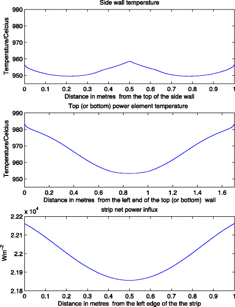

  

  Case 1: T _S =500°C

  Fig. 11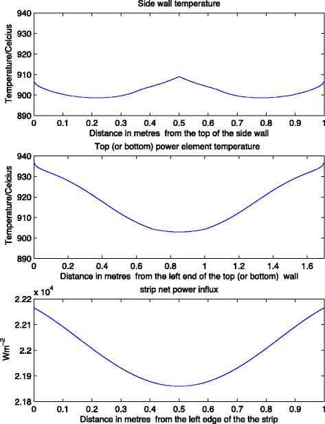

  

  Case 2: T _S =20°C

  Fig. 12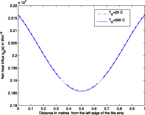

  

  The comparison of the net heat influx of the strip for T _S =500°C and T _S =20°C

Based on these results, we may calculate the strip temperature along the width by using the strip heat influx at T _S =500°C. The result is shown in Fig. 13. The temperature of the strip is seen to be varying smoothly with about 7°C in magnitude. The temperature variation would be about 1.2°C if the calculation was based on the isotherm model discussed in Section 3.3.

Fig. 13

The predicted temperature variation T _S across the strip width

Concluding remarks

We have analysed in detail two effects that contribute to extra heating of the steel strip at its edges.

The numerical results of Section 3 indicate that the geometrical effect due to view factors would account for an elevated temperature at the edges of about 7°C.

The analysis of Section 2 took into account the fact that the edges of the strip are really surfaces themselves. Although these surfaces are small, they contribute significantly to temperature increases at the edges because the rate of heat conduction away from the edges is slow. If one assumes that the edges are smooth and have an emissivity of about 0.2, the same as the larger surfaces of the steel, then this effect would result in temperature elevations of about 9°C at the edges. In reality the edges are much more rough than the rest of the strip’s surface. The actual temperature elevation is proportional to the emissivity, so an emissivity of 0.5, for example, would contribute to a temperature elevation of about 22°C near the edges. Moreover these elevated temperatures occur within about 1 cm of the edge of the strip, resulting in potentially damaging high temperature gradients.

References

Depree, N, Sneyd, J, Taylor, S, Taylor, MP, Chen, JJJ, Wang, S, O’Connor, M: Development and validation of models for annealing furnace control from heat transfer fundamentals. Comput. Chem. Eng. 34(11), 1849–1853 (2010).
Depree, N, Taylor, MP, Chen, JJJ, Sneyd, J, Taylor, S, Wang, S: Development of a three-dimensional heat transfer model for continuous annealing of steel strip. Ind. Eng. Chem. Res. 51(4), 1790–1795 (2012).
Howell, JR, Siegel, R: Thermal Radiation Heat Transfer. 5th. CRC Press, Boca Raton, Fla. (2011).
Incropera, FP, DeWitt, DP: Introduction to Heat Transfer. 4th. John Wiley and Sons, New York (2002).
McGuinness, M, Taylor, SW: Strip Temperature in a Metal Coating Line Annealing Furnace. In: Proceedings of the 2004 Mathematics-in-Industry Study Group (2004). http://www.maths-in-industry.org/miis/41/.
Modest, MF: Radiative Heat Transfer. 2nd edn. Academic Press, SAN DIEGO, CA (2003).
Pérez-Grande, I, Rivas, D, de Pablo, V: A global thermal analysis of multizone resistance furnaces with specular and diffuse samples. J. Crystal Growth. 246, 37–54 (2002).
Sauermann, H, Stenzel, CH, Keesmann, S, Bonduelle, B: High-stability control of multizone furnaces using optical fibre thermometers. Cryst. Res. Technol. 36(12), 1329–1343 (2001).
Teodorczyk, T, Januszkiewicz, KT: Computer simulation of electric multizone tube furnaces. Adv. Eng. Softw. 30, 121–126 (1999).
Zareba, S, Wolff, A, Jelali, M: Mathematical modelling and parameter identification of a stainless steel annealing furnace. Simul. Model. Prac. Theory. 60, 15–39 (2016).
Authors’ contributions
SWT was responsible for Section 2, SW was responsible for Section 3. Both authors read and approved the final manuscript.
Competing interests
The authors declare that they have no competing interests.
Publisher’s Note
Springer Nature remains neutral with regard to jurisdictional claims in published maps and institutional affiliations.
Author information
Authors and Affiliations
Corresponding author
Rights and permissions
Open Access This article is distributed under the terms of the Creative Commons Attribution 4.0 International License (http://creativecommons.org/licenses/by/4.0/), which permits unrestricted use, distribution, and reproduction in any medium, provided you give appropriate credit to the original author(s) and the source, provide a link to the Creative Commons license, and indicate if changes were made.
About this article
Cite this article
Taylor, S.W., Wang, S. Modelling steel strip heating within an annealing furnace. Pac. J. Math. Ind. 9, 5 (2017). https://doi.org/10.1186/s40736-017-0030-7
Received:
Accepted:
Published:
DOI: https://doi.org/10.1186/s40736-017-0030-7